How k2 calculates the transducer loss quickly
The new ASR toolkit k2/icefall gets great results while training models quickly. This is an explanation of how it does that by efficiently calculating the transducer loss and thereby using much less memory. Code is also shown.
If you’re new to transducers read this first for an excellent introduction: https://lorenlugosch.github.io/posts/2020/11/transducer/
Consider the training scenario. With CTC training your model will output a tensor (B,T,V) with B=’batch size’, T=’time steps’, and V=’vocab size’ (vocab size is the number of tokens your model can output). For each sample in a batch you can imagine a matrix where every traversing path represents an alignment (and CTC means you are summing across all of them). The following image shows an example with time on the x-axis, the tokens that should be output on the y. The path shown represents a particular sequence of token (diagonal) and blank (horizontal) that correspond to one alignment. Note that the probability distribution across V (the vocab) is, as long as you are at the same time-step, the same. In other words if you traverse vertically, the probability distribution across V does not change. It only changes if you traverse horizontally (by changing t).

This shows a specific alignment which can be repesented as a path through a matrix. Taken from the preprint linked at the bottom.
With transducer models this is different. Remember that the point of a transducer model is that you model P(y|x,y-1,y-2..) (instead of just P(y|x)), which means the token history matters. This means that you need an extra dimension (for the history) in the output tensor, and therefore you need a shape (B,T,U,V) with U = ‘tokens in reference’.
The way I imagine it is: Instead of a matrix representing different alignments for a single example, imagine stacked matrices (one behind the other), or a (3D) lattice. The z-axis goes along the stack and corresponds to the V dimension. Time is still on the x-axis, and the tokens that should be output still on y (this is the U dimension). This means that now for every combination of x,y (T,U) you have a different probability distribution across V.
This is a much larger tensor than the one CTC outputs! If the last paragraph was not clear, the main point is that the output tensor for transducers has shape (B,T,U,V) which is much larger than the output tensor of a CTC model which has shape (B,T,V).
Because it’s large, training is slow and uses a lot of memory. k2/icefall has created an approach for avoiding that!
The summary is one trains a simpler model to get bounds on what alignments are possible, and then uses those bounds to decrease the size of (B,T,U,V) to (B,T,S,V) (with S<<U ) and thereby efficiently train a model that models P(y|x,y-1,y-2..).
Now in more detail.
Let’s first review the normal method for creating the (B,T,U,V) tensor. This happens by combining the encoder and decoder outputs, which have shape (B,T,C) and (B,U,C). The combination is done by adding the two (with dimension unsqueezing so the result of the addition is (B,T,U,C)), and then projecting to (B,T,U,V).
Code:

The joiner that combines the encoder and decoder outputs. Note the dimension unsqueezing of the encoder and decoder outputs is assumed to have already happened (source code). The first projection you see just projects to a joiner dimension, `output_linear` projects to vocab size V.
Let’s just consider the case where B=1 (everything that follows holds true with B>1, this is just to simplify things) and we can work with the shape (T,U,V).
Remember our end-goal is to calculate the logprob of all alignments by summing across all of them. This requires stepping, from start to end, through each combination of time (T) and token history (U) in the (T,U,V) tensor. The first insight is that for training we don’t need to have a distribution across all tokens in V as we have a training transcript so we know at each position (T,U) the token probability that matters: In the first row on the y-axis (equals U axis, see figure at the start) it is the first token in U, in the second row it is the second token in U and so on. These token probabilities govern the vertical transitions, the horizontal transitions are dependent on the blank token probabilities. These probabilities are what we need (instead of a distribution across all).
Okay cool, but how do we actually get the logprobs we need for each position in (T,U,) without creating (T,U,V)?
This is done by initially treating the encoder and decoder as separate models that act as an AM and LM by modeling P(y|x) and P(y|y-1,y-2..). First the encoder and decoder outputs are projected to (T,V) and (U,V), then these are matrix-multiplied with V on the inner dimension to get a matrix (T,U) with marginalized values across V.
This lets us get normalized probabilities for tokens we care about: We can add together the unnormalized token log probabilities from the encoder and decoder, and subtract the marginalized value. In equation form (everything is in logprob here):
\[\log p(t,u,v)=l_{encoder}(t,v) + l_{decoder}(u,v) - l_{marginalized}(t,u)\]Because time and token history are independent of each other, we avoid having to create a (T,U,V) matrix.
Logprobs are used when adding, normal probs when multiplying (the previously mentioned matrix multiply), so the implementation has some exp() and log() calls.
Using the probabilities we efficiently calculate above, we create a matrix (T,U) containing the token probabilities we care about (those in the reference transcript), and additionally a matrix (T,U) with the blank probabilities (since blank transitions are always possible). We then calculate a simple transducer loss by using both matrices to traverse across (T,U) (we need both since we need non-blank token probs for vertical and blank for horizontal transitions) to find the logprob of all alignments.
Note you wouldn’t normally want to take this approach because the encoder and decoder outputs don’t get to interact before the token distribution is calculated (they’re added together after the projection to size V), as already mentioned this effectively uses separate AM and LM models (where the AM just sees audio and the LM just text). But the point of a transducer model is that you want an output P(y|x,y-1,y-2); something that directly conditions on both audio and text!
The idea here is to use the simple loss so that we can do a pruned version of the normal transducer loss. After some training with the simple loss the model will learn that some alignments (paths in (T,U)) are more or less likely than others.
This information can be used to set boundaries for each time step in T, which allows doing the proper transducer loss on a subset (T,S,V) with S<<U (because we know that for a given point in time only some tokens are possible, not all in U), which takes much less memory, is faster and trains the P(y|x,y_1) output. Effectively this means we are not considering all alignments, just those that are “reasonable” (according to the simple loss).
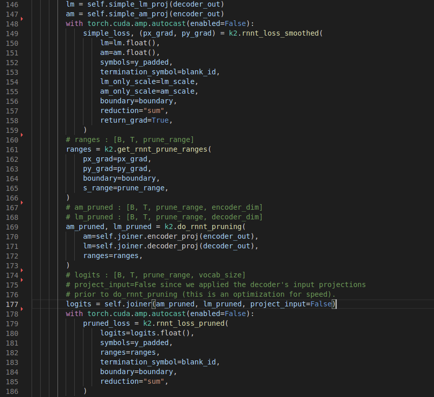
Let’s look at the high level code (I collapsed whitespace to make things more compact).
The following image shows all the steps to computing the pruned transducer loss. You can see the separate projection of encoder and decoder outputs to the vocab size, then computing a simple loss and using that (specifically the gradients) to get boundaries (here ranges) for creating (B,T,S,V) in logits. Finally the normal transducer loss is calculated. (source code)
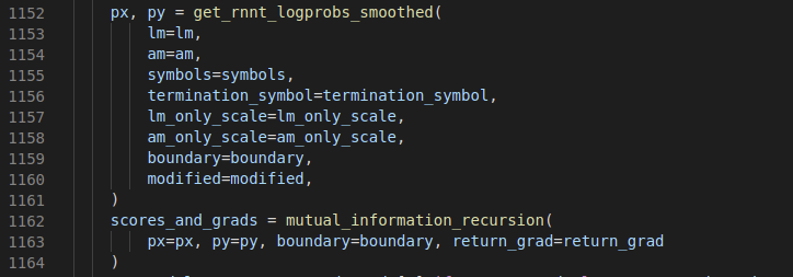
Looking slightly deeper into k2.rnnt_loss_smoothed we can see there are two stages: First calculating the matrix px (with shape (B,T,U,) of reference tokens) and matrix py (shape (B,T,U,) of blank token), then in mutual_information_recursion calculating the total logprob across all alignments ( source code ). Despite the intimidating name the implementation of the latter is quite straightforward (for CPU at least) and just involves doing the standard dynammic programming triple for-loop (for the batch, time, token dimensions), see here.
Thank you for reading, hope it is helpful, and please send an email / DM if something is unclear! :)
A preprint is available with nice results and additional details: https://arxiv.org/abs/2206.13236